Introduction
The independent t-test, also called the two sample t-test or student's t-test, is an inferential statistical test that determines whether there is a statistically significant difference between the means in two unrelated groups.
The independent-samples t-test (or independent t-test, for short) compares the means between two unrelated groups on the same continuous, dependent variable. For example, you could use an independent t-test to understand whether first year graduate salaries differed based on gender (i.e., your dependent variable would be "first year graduate salaries" and your independent variable would be "gender", which has two groups: "male" and "female"). Alternately, you could use an independent t-test to understand whether there is a difference in test anxiety based on educational level (i.e., your dependent variable would be "test anxiety" and your independent variable would be "educational level", which has two groups: "undergraduates" and "postgraduates").
Hypothesis for the Independent t-Test
The null hypothesis for the independent t-test is that the population means from the two unrelated groups are equal:
H0: u1 = u2 (Means of two groups are equal)
In most cases, we are looking to see if we can show that we can reject the null hypothesis and accept the alternative hypothesis, which is that the population means are not equal:
HA: u1 ≠ u2 (Means of two groups are not equal)
To do this, we need to set a significance level (alpha) that allows us to either reject or accept the alternative hypothesis. Most commonly, this value is set at 0.05.
What do we need to run an independent Test?
In order to run an independent t-test, you need the following:
Unrelated groups, also called unpaired groups or independent groups, are groups in which the cases in each group are different. Often we are investigating differences in individuals, which means that when comparing two groups, an individual in one group cannot also be a member of the other group and vice versa. An example would be gender - an individual would have to be classified as either male or female - not both.
Assumptions
When you choose to analyze your data using an independent t-test, part of the process involves checking to make sure that the data you want to analyze can actually be analyzed using an independent t-test. You need to do this because it is only appropriate to use an independent t-test if your data "passes" six assumptions that are required for an independent t-test to give you a valid result.
Do not be surprised if, when analyzing your own data, one or more of these assumptions is violated (i.e., is not met). This is not uncommon when working with real-world data rather than textbook examples, which often only show you how to carry out an independent t-test when everything goes well! However, don't worry. Even when your data fails certain assumptions, there is often a solution to overcome this. First, let's take a look at these six assumptions:
If you find that either one or both of your group's data is not approximately normally distributed and groups sizes differ greatly, you have two options:
(1) transform your data so that the data becomes normally distributed or
(2) run the Mann-Whitney U Test which is a non-parametric test that does not require the assumption of normality
Overcoming the violation of Homogeneity of Variance
If the Levene's Test for Equality of Variances is statistically significant, and therefore indicates unequal variances, we can correct for this violation by not using the pooled estimate for the error term for the t-statistic, and also making adjustments to the degrees of freedom using the Welch-Satterthwaite method. However, you can see the evidence of these tests as below:
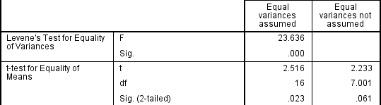
From the result of Levene's Test for Equality of Variances, we can reject the null hypothesis that there is no difference in the variances between the groups and accept the alternative hypothesis that there is a significant difference in the variances between groups. The effect of not being able to assume equal variances is evident in the final column of the above figure where we see a reduction in the value of the t-statistic and a large reduction in the degrees of freedom (df). This has the effect of increasing the p-value above the critical significance level of 0.05. In this case, we therefore do not accept the alternative hypothesis and accept that there are no statistically significant differences between means. This would not have been our conclusion had we not tested for homogeneity of variances.
How to use an Independent T-Test
This level assumes that you will use a software package to perform a t-test. If you want to know how to do it by hand, read level two. The result of using a t-test is that you know how likely it is that the difference between your sample means is due to sampling error. This is presented as a probability and is called a p-value. The p-value tells you the probability of seeing the difference you found (or larger) in two random samples if there is really no difference in the population.Generally, if this p-value is below 0.05 (5%), you can reject the null hypothesis and conclude that there is a statistically significant difference between the two population means. If you want to be particularly strict, you can decide that the p-value should be below 0.01 (1%). The level of p that you choose is called the significance level of the test. The p-value is calculated by first using the t-test formula to produce a t-value. This t-value is then converted to a probability either by software or by looking it up in a t-table. The next topic covers this part of the process
Calculating T Now we will look at the formula for calculating the t-value from an independent t-test. There are two versions of the formula, one for use when the two samples you wish to compare are of equal size, and one for differently sized samples. We will look at the first version because your data is equal in size for each sample and because it is the simpler formula. The unequal sized samples formula is shown in the extra topic section for your information.
The formula is the ratio of the difference between the two sample means to the variation within the two samples. The ratio has the following consequences:
Here is the formula to calculate the t value for equal sized Independent Samples

It reads: sample mean 1 minus sample mean 2 divided by the square root of (sample variance 1 plus sample variance 2, over n)
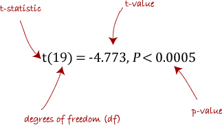
When reporting the result of an independent t-test, you need to include the t-statistic value, the degrees of freedom (df) and the significance value of the test (p-value). The format of the test result is: t(df) = t-statistic, p = significance value. Therefore, for the example above, you could report the result as t(7.001) = 2.233, p = 0.061.
For example
Inspection of Q-Q Plots revealed that cholesterol concentration was normally distributed for both groups and that there was homogeneity of variance as assessed by Levene's Test for Equality of Variances. Therefore, an independent t-test was run on the data as well as 95% confidence intervals (CI) for the mean difference. It was found that after the two interventions, It was found that after the two interventions, cholesterol concentrations in the dietary group exercise group (5.80 ± 0.38 mmol/L) (t(38) = 2.470, p = 0.018) with a difference of 0.35 (95% CI, 0.06 to 0.64) mmol/L.
Here is an example of Independent t-Test and how we perform with SAS
Key assumptions underlying the two-sample t-test are that the random samples are independent and that the populations are normally distributed with equal variances. (If the data are non-normal, then nonparametric tests such as the Mann-Whitney U are appropriate.)
SAS Syntax:
ODS HTML;
ODS GRAPHICS ON;
PROC TTEST DATA=FERT;
CLASS BRAND;
VAR HEIGHT;
Title 'Independent Group t-Test Example';
RUN;
ODS GRAPHICS OFF;
ODS HTML CLOSE;
QUIT;
This table helps you determine if the variances for the two groups are equal. If the p-value (Pr>F) is less than 0.05, you should assume UNEQUAL VARIANCES. In this case, the variances appear to be unequal.
Since p<.05, you can conclude that the mean for group B (43.8125) is statistically larger than the mean for group A (25.6429). More formally, you reject the null hypothesis that the means are equal and show evidence that they are different.

This graph provides a visual comparison of the means (and distributions) of the two groups. In this graph you can see that the mean of group B is larger than the mean of group A. You can also see why the test for equality of variances found that they were not the same (the variance for group A is smaller.)
A complete report of our result
In order to provide enough information for readers to fully understand the results when you have run an independent t-test, you should include the result of normality tests, Levene's Equality of Variances test, the two group means and standard deviations, the actual t-test result and the direction of the difference (if any). In addition, you might also wish to include the difference between the groups along with the 95% confidence intervals.
References
http://www.stattutorials.com/SAS/TUTORIAL-PROC-TTEST-2.htm
http://www.stattutorials.com/SAS/TUTORIAL-PROC-TTEST-INDEPENDENT.htm
The independent t-test, also called the two sample t-test or student's t-test, is an inferential statistical test that determines whether there is a statistically significant difference between the means in two unrelated groups.
The independent-samples t-test (or independent t-test, for short) compares the means between two unrelated groups on the same continuous, dependent variable. For example, you could use an independent t-test to understand whether first year graduate salaries differed based on gender (i.e., your dependent variable would be "first year graduate salaries" and your independent variable would be "gender", which has two groups: "male" and "female"). Alternately, you could use an independent t-test to understand whether there is a difference in test anxiety based on educational level (i.e., your dependent variable would be "test anxiety" and your independent variable would be "educational level", which has two groups: "undergraduates" and "postgraduates").
Hypothesis for the Independent t-Test
The null hypothesis for the independent t-test is that the population means from the two unrelated groups are equal:
H0: u1 = u2 (Means of two groups are equal)
In most cases, we are looking to see if we can show that we can reject the null hypothesis and accept the alternative hypothesis, which is that the population means are not equal:
HA: u1 ≠ u2 (Means of two groups are not equal)
To do this, we need to set a significance level (alpha) that allows us to either reject or accept the alternative hypothesis. Most commonly, this value is set at 0.05.
What do we need to run an independent Test?
In order to run an independent t-test, you need the following:
- One independent, categorical variable that has two levels (An independent variable, sometimes called an experimental or predictor variable, is a variable that is being manipulated in an experiment in order to observe the effect on a dependent variable, sometimes called an outcome variable)
- One dependent variable.
Unrelated groups, also called unpaired groups or independent groups, are groups in which the cases in each group are different. Often we are investigating differences in individuals, which means that when comparing two groups, an individual in one group cannot also be a member of the other group and vice versa. An example would be gender - an individual would have to be classified as either male or female - not both.
Assumptions
When you choose to analyze your data using an independent t-test, part of the process involves checking to make sure that the data you want to analyze can actually be analyzed using an independent t-test. You need to do this because it is only appropriate to use an independent t-test if your data "passes" six assumptions that are required for an independent t-test to give you a valid result.
Do not be surprised if, when analyzing your own data, one or more of these assumptions is violated (i.e., is not met). This is not uncommon when working with real-world data rather than textbook examples, which often only show you how to carry out an independent t-test when everything goes well! However, don't worry. Even when your data fails certain assumptions, there is often a solution to overcome this. First, let's take a look at these six assumptions:
- Assumption #1: The independent t-test requires that the dependent variable is approximately normally distributed within each group. We can test for this using a multitude of tests, but the Shapiro-Wilks Test or a graphical method, such as a Q-Q Plot, are very common. Your dependent variable should be measured on a continuous scale (i.e., it is measured at the interval or ratio level). Examples of variables that meet this criterion include revision time (measured in hours), intelligence (measured using IQ score), exam performance (measured from 0 to 100), weight (measured in kg), and so forth.
- Assumption #2: Your independent variable should consist of two categorical, independent groups. Example independent variables that meet this criterion include gender (2 groups: male or female), employment status (2 groups: employed or unemployed), smoker (2 groups: yes or no), and so forth.
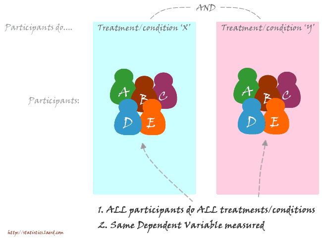
- Assumption #3: You should have independence of observations, which means that there is no relationship between the observations in each group or between the groups themselves. For example, there must be different participants in each group with no participant being in more than one group. This is more of a study design issue than something you can test for, but it is an important assumption of the independent t-test. If your study fails this assumption, you will need to use another statistical test instead of the independent t-test (e.g., a paired-samples t-test).
- Assumption #4: There should be no significant outliers. Outliers are simply single data points within your data that do not follow the usual pattern (e.g., in a study of 100 students' IQ scores, where the mean score was 108 with only a small variation between students, one student had a score of 156, which is very unusual, and may even put her in the top 1% of IQ scores globally). The problem with outliers is that they can have a negative effect on the independent t-test, reducing the validity of your results.
- Assumption #5: Your dependent variable should be approximately normally distributed for each group of the independent variable. We talk about the independent t-test only requiring approximately normal data because it is quite "robust" to violations of normality, meaning that this assumption can be a little violated and still provide valid results.
- Assumption #6: There needs to be homogeneity of variances. You can test this assumption using Levene’s test for homogeneity of variances. The independent t-test assumes the variances of the two groups you are measuring to be equal. If your variances are unequal, this can affect the Type I error rate. The assumption of homogeneity of variance can be tested using Levene's Test of Equality of Variances. If you have run Levene's Test of Equality of Variances, you will get a result similar to that below:This test for homogeneity of variance provides an F statistic and a significance value (p-value). We are primarily concerned with the significance level - if it is greater than 0.05, our group variances can be treated as equal. However, if p < 0.05, we have unequal variances and we have violated the assumption of homogeneity of variance.

If you find that either one or both of your group's data is not approximately normally distributed and groups sizes differ greatly, you have two options:
(1) transform your data so that the data becomes normally distributed or
(2) run the Mann-Whitney U Test which is a non-parametric test that does not require the assumption of normality
Overcoming the violation of Homogeneity of Variance
If the Levene's Test for Equality of Variances is statistically significant, and therefore indicates unequal variances, we can correct for this violation by not using the pooled estimate for the error term for the t-statistic, and also making adjustments to the degrees of freedom using the Welch-Satterthwaite method. However, you can see the evidence of these tests as below:
How to use an Independent T-Test
This level assumes that you will use a software package to perform a t-test. If you want to know how to do it by hand, read level two. The result of using a t-test is that you know how likely it is that the difference between your sample means is due to sampling error. This is presented as a probability and is called a p-value. The p-value tells you the probability of seeing the difference you found (or larger) in two random samples if there is really no difference in the population.Generally, if this p-value is below 0.05 (5%), you can reject the null hypothesis and conclude that there is a statistically significant difference between the two population means. If you want to be particularly strict, you can decide that the p-value should be below 0.01 (1%). The level of p that you choose is called the significance level of the test. The p-value is calculated by first using the t-test formula to produce a t-value. This t-value is then converted to a probability either by software or by looking it up in a t-table. The next topic covers this part of the process
Calculating T Now we will look at the formula for calculating the t-value from an independent t-test. There are two versions of the formula, one for use when the two samples you wish to compare are of equal size, and one for differently sized samples. We will look at the first version because your data is equal in size for each sample and because it is the simpler formula. The unequal sized samples formula is shown in the extra topic section for your information.
The formula is the ratio of the difference between the two sample means to the variation within the two samples. The ratio has the following consequences:
- When the difference between the sample means is large and the variation within each sample is small, t is large;
- When the difference between the sample means is small and the variation within each sample is large, t is small.
Here is the formula to calculate the t value for equal sized Independent Samples
It reads: sample mean 1 minus sample mean 2 divided by the square root of (sample variance 1 plus sample variance 2, over n)
- x1 is read as x1-bar and is the mean of the first sample;
- x2 is read as x2-bar and is the mean of the second sample;
- The variance is the standard deviation squared (hence s2).
- The subscript numbers (1 and 2 to the bottom right of the x and s in the formula) refer to sample 1 and sample 2;
When reporting the result of an independent t-test, you need to include the t-statistic value, the degrees of freedom (df) and the significance value of the test (p-value). The format of the test result is: t(df) = t-statistic, p = significance value. Therefore, for the example above, you could report the result as t(7.001) = 2.233, p = 0.061.
For example
Inspection of Q-Q Plots revealed that cholesterol concentration was normally distributed for both groups and that there was homogeneity of variance as assessed by Levene's Test for Equality of Variances. Therefore, an independent t-test was run on the data as well as 95% confidence intervals (CI) for the mean difference. It was found that after the two interventions, It was found that after the two interventions, cholesterol concentrations in the dietary group exercise group (5.80 ± 0.38 mmol/L) (t(38) = 2.470, p = 0.018) with a difference of 0.35 (95% CI, 0.06 to 0.64) mmol/L.
Here is an example of Independent t-Test and how we perform with SAS
When data are collected on subjects where subjects are (hopefully randomly) divided into two groups, this is called an independent or parallel study. That is, the subjects in one group (treatment, etc) are different from the subjects in the other group.
The SAS PROC TTEST procedure
This procedure is used to test for the equality of means for a two-sample (independent group) t-test. For example, you might want to compare males and females regarding their reaction to a certain drug, or one group who receives a treatment compared to another that receives a placebo. The purpose of the two-sample t-test, is to determine whether your data provide you with enough evidence to conclude that there is a difference in mean reaction levels between the two group. In general, for a two-sample t-test you obtain independent random samples of size N1 and N2 and from the two populations of interest, and then you compare the observed sample means.
The typical hypotheses for a two-sample t-test are
Ho: m1 = m2 (means of the two groups are equal)
Ha: m1¹ m2 (means are not equal)
Ha: m1¹ m2 (means are not equal)
Key assumptions underlying the two-sample t-test are that the random samples are independent and that the populations are normally distributed with equal variances. (If the data are non-normal, then nonparametric tests such as the Mann-Whitney U are appropriate.)
SAS Syntax:
Simplified syntax for the TTEST procedure is
PROC TTEST <options>;
CLASS variable; <statements>;
RUN;
PROC TTEST <options>;
CLASS variable; <statements>;
RUN;
Common OPTIONS:
- DATA = datasetname: Specifies what data set to use.
- COCHRAN: Specifies that the Cochran and Cox probability approximation is to be used for unequal variances.
- CLASS statement: The CLASS statement is required, and it specifies the grouping variable for the analysis.
The data for this grouping variable must contain two and only two values. An example PROC TTEST command is
PROC TTEST DATA=MYDATA;
CLASS GROUP;
VAR SCORE;
RUN;
In this example, GROUP contains two values, say 1 or 2. A t-test will be performed on the variable SCORE.
- VAR variable list;: Specifies which variables will be used in the analysis.
- BY variable list;: (optional) Causes t-tests to be run separately for groups specified by the BY statement.
EXAMPLE:
A biologist experimenting with plant growth designs an experiment in which 15 seeds are randomly assigned to one of two fertilizers and the height of the resulting plant is measured after two weeks. She wants to know if one of the fertilizers provides more vertical growth than the other.
STEP 1. Define the data to be used. (If your data is already in a data set, you don't have to do this step). For this example, here is the SAS code to create the data set for this experiment:
DATA FERT;
INPUT BRAND $ HEIGHT;
DATALINES;
A 20.00
A 23.00
A 32.00
A 24.00
A 25.00
A 28.00
A 27.50
B 25.00
B 46.00
B 56.00
B 45.00
B 46.00
B 51.00
B 34.00
B 47.50
;
RUN;
INPUT BRAND $ HEIGHT;
DATALINES;
A 20.00
A 23.00
A 32.00
A 24.00
A 25.00
A 28.00
A 27.50
B 25.00
B 46.00
B 56.00
B 45.00
B 46.00
B 51.00
B 34.00
B 47.50
;
RUN;
STEP 2. The following SAS code specifies a two-sample t-test using the FERT dataset.(NOTE: For SAS 9.3, you don't need the ODS statements.)
ODS HTML;
ODS GRAPHICS ON;
PROC TTEST DATA=FERT;
CLASS BRAND;
VAR HEIGHT;
Title 'Independent Group t-Test Example';
RUN;
ODS GRAPHICS OFF;
ODS HTML CLOSE;
QUIT;
The CLASS statement specifies the grouping variables with 2 categories (in this case A and B).
The VAR statement specifies which variable is the observed (outcome or dependent) variable.
Interpret the output. The (abbreviated) output contains the following information
| BRAND | N | Mean | Std Dev | Std Err | Minimum | Maximum |
|---|---|---|---|---|---|---|
| A | 7 | 25.6429 | 3.9021 | 1.4748 | 20.0000 | 32.0000 |
| B | 8 | 43.8125 | 9.8196 | 3.4717 | 25.0000 | 56.0000 |
| Diff (1-2) | -18.1696 | 7.6778 | 3.9736 |
This first table provides means, sd, min and max for each group and the mean difference.
| BRAND | Method | Mean | 95% CL Mean | Std Dev | 95% CL Std Dev | ||
|---|---|---|---|---|---|---|---|
| A | 25.6429 | 22.0340 | 29.2517 | 3.9021 | 2.5145 | 8.5926 | |
| B | 43.8125 | 35.6031 | 52.0219 | 9.8196 | 6.4925 | 19.9855 | |
| Diff (1-2) | Pooled | -18.1696 | -26.7541 | -9.5852 | 7.6778 | 5.5660 | 12.3692 |
| Diff (1-2) | Satterthwaite | -18.1696 | -26.6479 | -9.6914 | |||
The next table provides 95% Confidence Limits on both the means and Standard Deviations, and the mean difference using both the pooled (assume variances are equal) and Satterthwaite (assume variances are not equal) methods.
Before deciding which version of the t-test is appropriate, look at this table
| Equality of Variances | ||||
|---|---|---|---|---|
| Method | Num DF | Den DF | F Value | Pr > F |
| Folded F | 7 | 6 | 6.33 | 0.0388 |
This table helps you determine if the variances for the two groups are equal. If the p-value (Pr>F) is less than 0.05, you should assume UNEQUAL VARIANCES. In this case, the variances appear to be unequal.
Therefore... in the t-test table below (for this case) choose the Satterthwaite t-test, and report a p-value of p=0.0008. If the variances were assumed equal, you would report the Pooled variances t-test.
| Method | Variances | DF | t Value | Pr > |t| |
|---|---|---|---|---|
| Pooled | Equal | 13 | -4.57 | 0.0005 |
| Satterthwaite | Unequal | 9.3974 | -4.82 | 0.0008 |
Since p<.05, you can conclude that the mean for group B (43.8125) is statistically larger than the mean for group A (25.6429). More formally, you reject the null hypothesis that the means are equal and show evidence that they are different.
When you use the ODS GRAPHICS ON option, you get the following graph:
This graph provides a visual comparison of the means (and distributions) of the two groups. In this graph you can see that the mean of group B is larger than the mean of group A. You can also see why the test for equality of variances found that they were not the same (the variance for group A is smaller.)
A complete report of our result
In order to provide enough information for readers to fully understand the results when you have run an independent t-test, you should include the result of normality tests, Levene's Equality of Variances test, the two group means and standard deviations, the actual t-test result and the direction of the difference (if any). In addition, you might also wish to include the difference between the groups along with the 95% confidence intervals.
References
http://www.stattutorials.com/SAS/TUTORIAL-PROC-TTEST-2.htm
http://www.stattutorials.com/SAS/TUTORIAL-PROC-TTEST-INDEPENDENT.htm